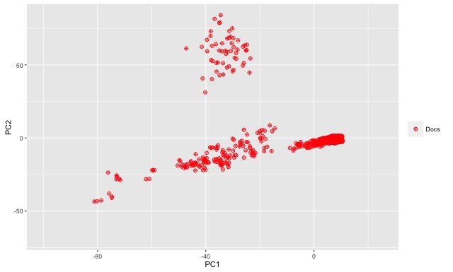
We finished Part One of this blog post with a simplified example to demonstrate how one might be able to measure document similarity across a given corpus using a document-term matrix as a starting point. Let’s now turn back to R and our larger sample data set. As an exploratory step we can visualize the document-term matrix within a two-dimensional space. We can use a principal component analysis to summarize the variation within the data and then generate a plot of just the first two principal components. Each of the two principal components represents a grouping of the most relevant variables in describing how documents are distributed across the n-dimensional space. Using the first two principal components as our axes, we get the two-dimensional plot displayed at the beginning of this post (above), which represents a rough distribution of our documents.
Given the way our data was selected, this distribution makes at least some sense. Remember that the first 300 or so documents were selected based on a targeted proximity search (i.e. fantasy w/5 football), whereas I selected the remaining documents randomly from a much larger portion of the Enron data set. The PCA plot clearly shows two groups of documents.
To accomplish our near-duplicate analysis we can utilize an agglomerative hierarchical clustering analysis against the document-term matrix. In short, an agglomerative hierarchical clustering analysis starts by assigning every document its own cluster and then merges the closest (i.e. the most similar) clusters into one cluster and repeats the process until all clusters have merged into one single cluster. The distance between each cluster is calculated at each step and this distance is how we determine similarity.
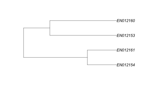
Having run the analysis on just the document-term matrix we can visualize it as a tree diagram (a dendrogram). For example, here is a dendrogram of just four very similar documents from the our sample data set. A close comparison shows that while all four are quite similar, EN012160 is slightly more similar to EN012153 than it is to EN012161.
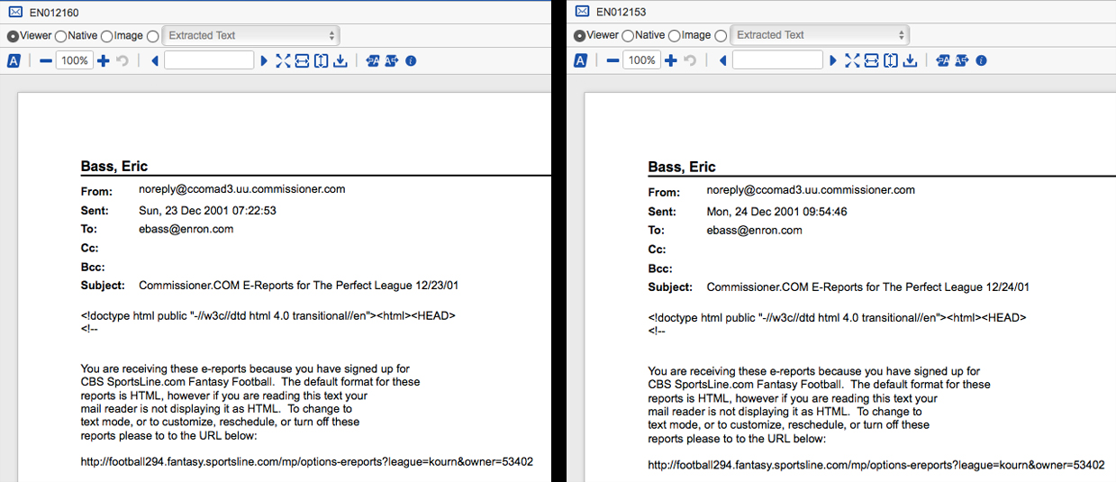
Here is a side-by-side comparison of EN012160 and EN012153. They are nearly identical, but not exactly the same. Because of the slight differences these two documents would never dedupe based on hash values. They are, however, so similar that we may want to treat them the same for review purposes. That is, we may want to be able to identify them as near-duplicates of each other and apply the same coding decisions to them. This is the advantage of near-duplicate identification. It’s an automated process for grouping similar documents with similar documents, which when combined with a sensible review workflow can save you time and money by accelerating review and improving QC. As an interesting aside, note that there are differences in the dates. Remember that we removed numbers during our preprocessing and, therefore, those dates are not being considered in our near-duplicate analysis in R.
Here is a side-by-side comparison of EN012160 and EN012161 showing the slight variation in the email subjects.

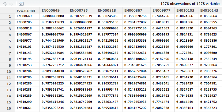
Using R we can output a CSV that contains the original Document Identifier and corresponding near-duplicate group IDs for each document within the corpus. The group a particular document belongs to is determined based off of its relative distance from other documents within the corpus. That is, documents that are very close to each other will belong to the same group. After generating the distance matrix in R we can view the results as a matrix.
Pictured below are documents and their relative distances to each other. You can observe that when a document is compared to itself the relative distance is 0. Moreover, if you compare some documents to others you can observe where some documents are very similar to each other versus where some documents are very different. For example, you can deduce that EN000649 is more similar to EN000785 than it is to EN009977 because the relative distance between EN000649 and EN009977 is almost twice that of EN000649 and EN000785.
Another way you can visualize this step is to turn back to the dendrogram and imagine slicing it at a point between the end tips (which represent individual documents) and the largest cluster (the cluster containing every document). Slicing the dendrogram right at the tips would result in every document being assigned to its own group, which isn’t what we want. Instead we want there to be some document grouping where document similarity is very high. If you slice it at a point a little bit farther up the tree you can identify clusters of documents that are very similar to each other.
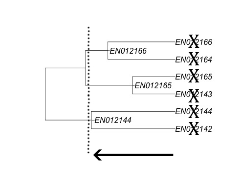
In the above picture, slicing the tree where illustrated by the dotted line would result in creating three near-duplicate groups comprised of six documents, named based on the most inclusive document. Once you have exported the CSV you can then overlay the information back into Relativity as a relational field and your near-duplicate analysis is done. The relevant near-duplicate group ID field your system uses to identify near-duplicates should be populated with the data you generated in R and Relativity will do the rest.

Our analysis using R, a free and open-source language, produces results that are comparable to what you might expect from other à la carte near-duplicate tools. For example, the output generated using LexisNexis’ LAW PreDiscovery grouped documents in pretty much the same manner as what we generated using R. Of course, the methods we discussed today are not the only way to perform near-duplicate identification and there are certainly issues with scalability, but hopefully you found this overview informative.
Below you can download the CSV outputs from our near-duplicate identification using R and LexisNexis’ own paid tool. The results do differ from one another, but a comparison shows that the two methods have largely grouped documents in the same way. There are certainly differences, which we can speculate about. For example, I imagine LexisNexis’ tool considers numbers in its near-duplicate analysis while ours did not (remember we removed numbers when we pre-processed our data). Another area where they differ would likely be how the “master document” is determined. LexisNexis is not clear as to exactly how their process identifies the master document, but it does appear to be more complicated than the way I did it. In the R program I created the master document is determined simply by choosing whatever document has the most content (i.e. a simple character count), the theory being that the largest document among similar documents should be the one all others are compared to. If you would like to compare results from both approaches download the attached .zip file.
I guarantee any salesperson you speak with from any eDiscovery vendor will tell you their product is better than another’s because (insert marketing jargon here), but the reality is that the underlying technology, while complex, isn’t so mindbogglingly difficult – in the end it’s just data and math. The starting point is always just document content (and often specific metadata fields). While my approach is very rudimentary, it still performs well enough to be useful in the real world (remember, it’s free).
Hopefully these blog posts have improved your understanding about how near-duplicate identification technology can work. Digging into the statistical underpinnings of a tool and not blindly accepting the technology to be a black box will ultimately help you be a better eDiscovery professional. For example, what concerns would you have if attempting to perform a near-duplicate analysis on produced hardcopy (i.e. scanned paper documents) data?
In a future blog post I will write about how we can use R to perform one of the more advanced forms of technology-assisted review being used today. Specifically, we will use R to build a latent semantic index and then use machine learning categorization techniques to make our own rudimentary “predictive coding” software.