Near-duplicate identification is one of the more common textual analytics tools used in eDiscovery. Not to be confused with document deduplication, which relies on hash values, near-duplicate identification calculates document similarity based off textual content. For example, if you had two documents containing exactly the same text – one being a native email file and the other being a PDF version of that same email – the hash values of the two files would be entirely different. However, near-duplicate identification looks at just the textual content of the two documents and can determine that they are very similar to each other. This can accelerate document review and improve accuracy.
There are a number of ways we can use near-duplicate identification to accelerate any eDiscovery review project. Near-duplicate identification can be used in conjunction with bulk coding or coding propagation to effectively review large swaths of documents at once. The big assumption is that documents that are very similar to each other should be categorized in the same manner. Near-duplicate identification can also be a powerful QC tool. For example, let’s say your review team has identified a subset of privileged documents within a review data set and you are concerned that other privileged documents may have been missed. You could isolate all documents coded as being privileged and then isolate all near-duplicates of those documents not coded as being privileged for immediate re-review.

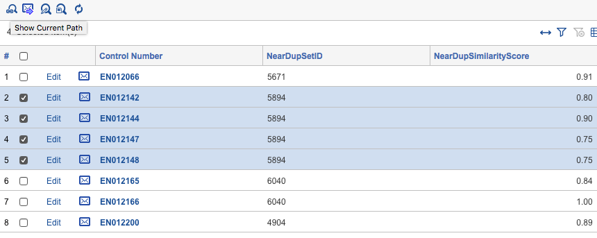
Most near-duplicate identification tools require the input of document text and output a few fields such as a near-duplicate group ID and near-duplicate similarity score. The near-duplicate group ID is how any eDiscovery review platform knows two documents are similar, with similar documents sharing the same near-duplicate group ID. The near-duplicate similarity score is usually a decimal or percentage value, which indicates how similar a given document is to a near-duplicate group’s primary document (i.e. the document in the near-duplicate group that other documents are being compared to). In the example screenshot below EN012142, EN012144, EN012147, and EN012148 all belong to the near-duplicate group ID 5894 with varying similarity scores.
To my surprise, there seems to be a lot of confusion among credentialed eDiscovery professionals about exactly what near-duplicate detection entails. I’m not entirely sure why this is the case, but I think it has at least something to do with the fact that the vendors and software developers that create these tools don’t spent too much time explaining exactly how their products work, making it a “black box” tool to the user. This isn’t exactly a surprise, I suppose.
I thought it would be fun and instructive to come up with my own way to perform near-duplicate identification analysis, for free, that performs similar to the paid solutions offered by companies such as Equivio, Brainspace, kCura Relativity Analytics, LexisNexis, etc. I gave myself two requirements. First, the near-duplicate analysis needed to work. Second, because I primarily use Relativity I wanted my approach to be able to easily handle an input an end user could easily export from any Relativity environment and generate an output that an end user would be able to overlay back into any Relativity environment.
Coming up with a solution.
I know at least a few people that know about R programming language so naturally that is where I looked. There’s nothing special or unique about R besides the fact that it’s free, open source, and generally awesome. I would suggest anyone give it a look, as it’s not as complicated as it may seem and there are resources everywhere online that will help you when needed. You should also install RStudio. RStudio is an integrated development environment (IDE), a feature-rich user interface, which will make your life much easier.
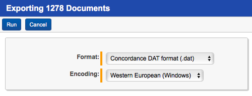
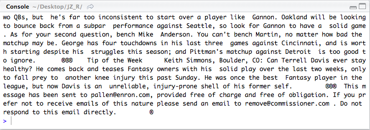
Before we do anything in R we need to get our data. The first step involves exporting your data out of Relativity. R can work with just about anything and I’ve done the same analysis with just document-level text files. For this post I found it easiest to export the data you need as a DAT. Isolate the universe of documents you want run your near-duplicate analysis on in Relativity as a saved search. For this data set I chose 1278 documents from the Enron data set in the following manner:
- the first 300 or so are documents that hit on the dtSearch term: fantasy w/5 football;
- the remainder were selected randomly from the greater Enron data set.
You can download the DAT I used for this post here. Your DAT file must have the following fields, whatever your own Relativity environment calls them: Unique Document Identifier and Extracted Text. The Extracted Text is what you’re going to run the near-duplicate analysis against and the Control Number is how you tie it back to the original document on the system. Because you’re running an analysis on the extracted text it should go without saying that documents with very little or no text will not analyze very well and it’s a good idea to exclude them. Here, I’ve exported a DAT containing documents selected from the Enron data set.
Once you have RStudio open and your working directory set, load the package(s) you’re going to use. Packages are collections of functions and code. For this demo we’re just going to need the R package tm, which has all of the tools we’re going to use.
Next, we create our corpus based off of the DAT we exported from Relativity. The code below will create a data frame, df, from the DAT. You will need to specify the delimiter and quote characters to be consistent with what’s in your DAT. For example, pilcrow [¶] and thorn [þ] are often recommended as comma and quote, respectively.
df <- read.table(allowEscapes = TRUE,”Sample.dat”, sep = “YOURSEPERATOR”, quote = “YOURQUOTE”, header = TRUE, encoding = “latin1”, stringsAsFactors=F) #reads in the DAT
We then create the text corpus from the Extracted.Text within the data frame.
my.corpus <- Corpus(VectorSource(df$”Extracted.Text”)) #creates corpus from the Extracted.Text field.
Next we are going to use some of the functions built into the tm package to pre-process the corpus. Pre-processing your corpus is extremely important because it lets you clean up the data by removing unwanted and unneeded text, which will ultimately lead to a faster and more accurate near-duplicate analysis.
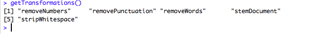
Typing in getTransformations() in the R prompt will return a list of the available transformation functions. Specifically, we are going to remove numbers, remove punctuation, remove stop words, remove white space, and stem all of the words within the corpus. Think of it as refining your data.
You can watch how each transformation changes the content of an individual document to get a better understanding of what you’re actually doing. To view the contents of an individual document (here, document 3), execute the following code:
writeLines(as.character(my.corpus[[3]]))
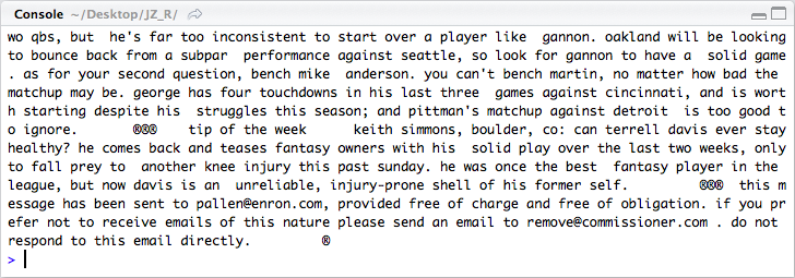
First we are going to transform all text to lower case. R is case-sensitive and we do not want R to differentiate between words based on capitalization alone (i.e. we want “Good” and “good” to be counted just as “good”).
my.corpus <- tm_map(my.corpus, content_transformer(tolower))
Note the changes to the third document in our corpus. Capitalized letters have been converted to lower case.
Next, we remove numbers from our corpus. While there may certainly be instances where you may want to keep numbers, we are removing them here.
my.corpus <- tm_map(my.corpus, removeNumbers)
Next, we remove punctuation.
my.corpus <- tm_map(my.corpus, removePunctuation)
Next, we remove stop words. The tm package has its own stop word list, which can be customized if needed. Stop words are words that are very commonly used and, therefore, are not especially useful for measuring document relationships. If a word occurs in every single document (common words like “the,” “and,” etc.) it’s not a unique characteristic that helps us tell one document from another.
my.corpus <- tm_map(my.corpus, removeWords, stopwords(“english”))
Next we remove any extra white space within the corpus.
my.corpus <- tm_map(my.corpus, stripWhitespace)
Finally, we are going to stem all of the words in the document. Again, the tm package has its own stemming function. Stemming boils words down to their root based on word tables. For example, the words obligation, obligated, obliged, etc. would be reduced to just “oblig.”
my.corpus <- tm_map(my.corpus, stemDocument)
Note what the final version of the third document in our corpus looks like.
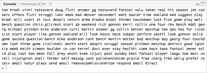
Having applied the above transformations we now have a much cleaner corpus. We’re ready to create the document-term-matrix.
my.dtm <- DocumentTermMatrix(my.corpus)
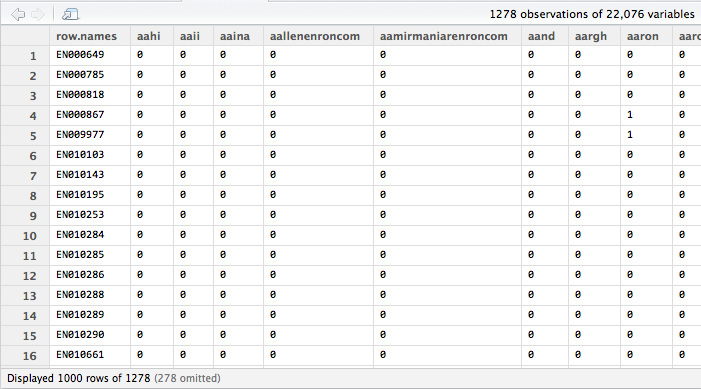
The document-term matrix is just a two-dimensional array that represents your entire corpus. Think of it as an Excel spreadsheet. Each row represents a document; each column represents a term; each cell contains a number, which indicates how many times that word occurs in the corresponding document. It’s an m-by-n matrix. Based off of our sample data the resulting document-term matrix is a 1,278 by 22,076 matrix. That’s a lot of dimensions given our small data set and if we were dealing with hundreds of thousands or millions of documents we would need to come up with ways to reduce dimensionality, but that’s a problem for another day.
A simplified example.
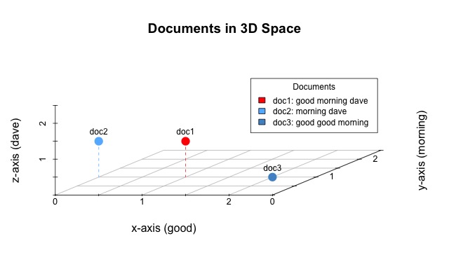
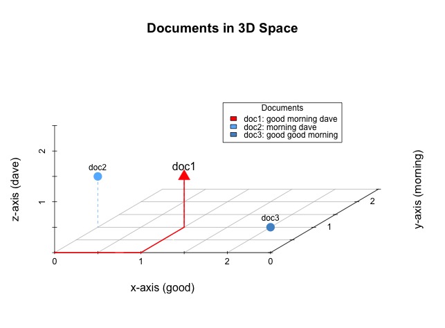
It’s understandably difficult to visualize our entire corpus based on the document-term matrix alone with so many dimensions. So let’s break here and think about a very simple example. Consider a different corpus of just three documents containing the following text:
doc1: “good morning dave”
doc2: “morning dave”
doc3: “good good morning”
We can represent these three documents as the following document-term matrix:
| good | morning | dave | |
| doc1 | 1 | 1 | 1 |
| doc2 | 0 | 1 | 1 |
| doc3 | 2 | 1 | 0 |
Just as with our larger document-term matrix each row represents a document and each column represents a unique word within the corpus. We can visualize the documents within an n-dimensional space. Fortunately, there are only three unique words in our simplified corpus and, therefore, we need only three dimensions to represent it. Here is a visual representation of our three documents, as they might exist in a three-dimensional space.
Imagine yourself standing in a room. To get to the location occupied by doc1, containing the words good, morning, and dave, you would need to take one step along the x-axis, one step along the y-axis, and then one step up the z-axis. The next visualization should be fairly self-explanatory. For example, doc 1 is a point located at (x=1,y=1,z=1) because it contains one of each of the words: good, morning, and dave. Likewise, the other documents occupy locations that equate to their own word contents.
Given a corpus of documents perhaps the simplest way we can gauge document similarity is based off of the distance between them. The Euclidean distance (e.g. ordinary, as the crow flies, or straight-line distance) is the distance between two points or, here, documents since that is what the points represent. The distance between doc1 and doc3 is the length of the line connecting the two.
You could calculate the Euclidean distance between doc1 and doc3 using the following formula:
![]()
Likewise, you can calculate the distance between points occupying an n-dimensional space in very much the same way as you would for documents occupying a three-dimensional space. The formula would be:
![]()
The Euclidean distance is just one distance measurement and there are certainly better ones to use under different circumstances (e.g. Manhattan distance, Pearson Correlation distance, etc.), but I’m using it here as a simple example.
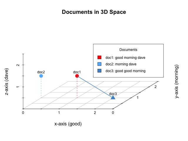
In the above image, the blue line between doc1 and doc3 has a distance of 1.41. While that doesn’t mean very much on its own, the important takeaway is that we have just quantified the relationship between two documents. Now scale this up to a much, much larger corpus and you can see how we are able to discern document similarity based on a document-term matrix, which is based on just the textual content of each document within the entire corpus. Points that occupy similar locations within the n-dimensional space (i.e. have a small distance between them) will represent documents that contain the same words and, therefore, are similar to each other. That’s the idea, at least.
Part Two of this post will return to our sample data set and discuss how we can actually go about generating a usable output that could be loaded back into a Relativity review environment.